
This vignette demonstrates three very simple analysis workflows using thesis metadata from the NTC. Each example starts with data collection and ends with a table or plot. The workflows cover research trends, institutional comparisons, and keyword mining.
The vignette does not run live NTC queries during ordinary package
builds. It uses representative output so readers can see each workflow
without depending on the live portal. Set
TEZR_LIVE_EXAMPLES=true before rendering if you want to
execute the portal requests.
Prerequisites: Familiarity with dplyr and ggplot2. See the Getting Started vignette for search function details.
library(tezr)
library(dplyr)
library(ggplot2)
library(tidyr)
library(stringr)

rolling_mean_right <- function(x, k) {
  vapply(seq_along(x), function(i) {
    if (i < k) {
      return(NA_real_)
    }
    mean(x[(i - k + 1):i])
  }, numeric(1))
}
Example 1: Research Trends Over Time
Suppose you want to track how interest in a topic has changed across decades. This is a standard starting point for bibliometric analysis. You can replace the search term with your own topic of interest.
Collecting Data
Let’s use search_advanced() with the
search_field parameter set to all. The result is a tibble
of matching records with year, author, university, and other
metadata.
# Search for "iklim değişikliği" (climate change) in thesis titles
if (live_examples) {
  climate <- search_advanced(keyword = "iklim değişikliği",
                             search_field = "all",
                             max_search_results = Inf)
} else {
  climate <- tezr_example_climate_results()
}
glimpse(climate)
#> Rows: 24
#> Columns: 13
#> $ thesis_no         <chr> "9677551", "9759882", "9557793", "9749764",…
#> $ title_original    <chr> "Iklim degisikligi 1", "Iklim degisikligi 2…
#> $ title_translation <chr> "Climate change 1", "Climate change 2", "Cl…
#> $ author            <chr> "PERIHAN EZGI BALLI", "CENAP ALAYBEYI", "SE…
#> $ university        <chr> "Ankara Universitesi", "Istanbul Universite…
#> $ year              <int> 2015, 2016, 2017, 2018, 2019, 2020, 2021, 2…
#> $ thesis_type_tr    <chr> "Doktora", "Yuksek Lisans", "Yuksek Lisans"…
#> $ thesis_type_en    <chr> "Master", "Doctorate", "Master", "Doctorate…
#> $ language_tr       <chr> "Turkce", "Turkce", "Turkce", "Turkce", "Tu…
#> $ language_en       <chr> "Turkish", "Turkish", "Turkish", "Turkish",…
#> $ subject_tr        <chr> "Cevre Bilimleri; Ekonomi", "Cevre Bilimler…
#> $ subject_en        <chr> "Environmental Sciences; Economics", "Envir…
#> $ detail_id         <chr> "TCKf4ksTOVsOBqUcPYMKWQ", "LypZzbdoWcG0f3c6…
Yearly Counts with Rolling Average
Let’s count theses per year and smooth with a 10-year rolling
average. The rolling average reveals sustained growth versus one-off
spikes. We can adjust k for a wider or narrower window.
# Count theses per year
yearly_counts <- climate |>
  count(year) |>
  arrange(year) |>
  mutate(
    year_numeric = as.numeric(year),
    # 10-year rolling average to smooth yearly variation
    rolling_avg = rolling_mean_right(n, k = 10)
  )

# Bar chart with rolling average overlay
yearly_counts |>
  na.omit() |>
  ggplot(aes(x = year_numeric)) +
  geom_col(aes(y = n), fill = "steelblue", alpha = 0.6) +
  geom_line(aes(y = rolling_avg), color = "red", linewidth = 1) +
  labs(
    title = "Climate Change Research in Turkish Universities",
    subtitle = "Annual thesis count with 10-year rolling average",
    x = "Year",
    y = "Number of Theses",
    caption = "Red line: 10-year moving average"
  ) +
  theme_minimal(base_size = 11)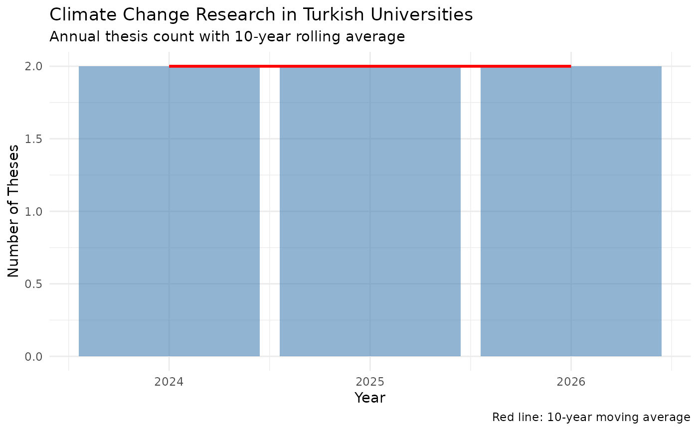
Master’s vs PhD Trends
We can split by degree type to see what drives growth. Filter to the two main types for a readable plot.
# Compare master's and PhD thesis counts over time
type_trends <- climate |>
  filter(thesis_type_en %in% c("Master", "Doctorate")) |>
  count(year, thesis_type_en) |>
  mutate(year = as.numeric(year))

type_trends |>
  ggplot(aes(x = year, y = n, color = thesis_type_en)) +
  geom_line(linewidth = 1) +
  labs(
    title = "Climate Research by Degree Type",
    x = "Year",
    y = "Number of Theses",
    color = "Degree"
  ) +
  theme_minimal(base_size = 11)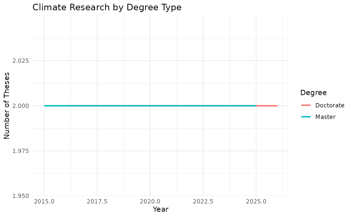
Example 2: Comparing Universities
Suppose we want to identify which universities produce the most
research in a given field. You can replace "Ekonometri"
with any subject from list_subjects().
Collecting University-Level Data
# All econometrics theses, counted by university
if (live_examples) {
  econ_theses <- search_detailed(subject = "Ekonometri",
                                 max_search_results = Inf)
} else {
  econ_theses <- tezr_example_econ_theses()
}

uni_counts <- econ_theses |>
  count(university, sort = TRUE)

uni_counts |>
  head(10)
#> # A tibble: 4 × 2
#>   university                n
#>   <chr>                 <int>
#> 1 Ankara Universitesi       4
#> 2 Ege Universitesi          4
#> 3 Istanbul Universitesi     4
#> 4 Marmara Universitesi      4
Top Universities Bar Chart
Let’s create a simple bar chart. Horizontal bars make long Turkish university names easy to read.
uni_counts |>
  head(10) |>
  ggplot(aes(x = n, y = reorder(university, n))) +
  geom_col() +
  labs(
    title = "Top 10 Universities for Econometrics Research",
    subtitle = "Total thesis count (all years)",
    x = "Number of Theses",
    y = NULL
  ) +
  theme_minimal(base_size = 11)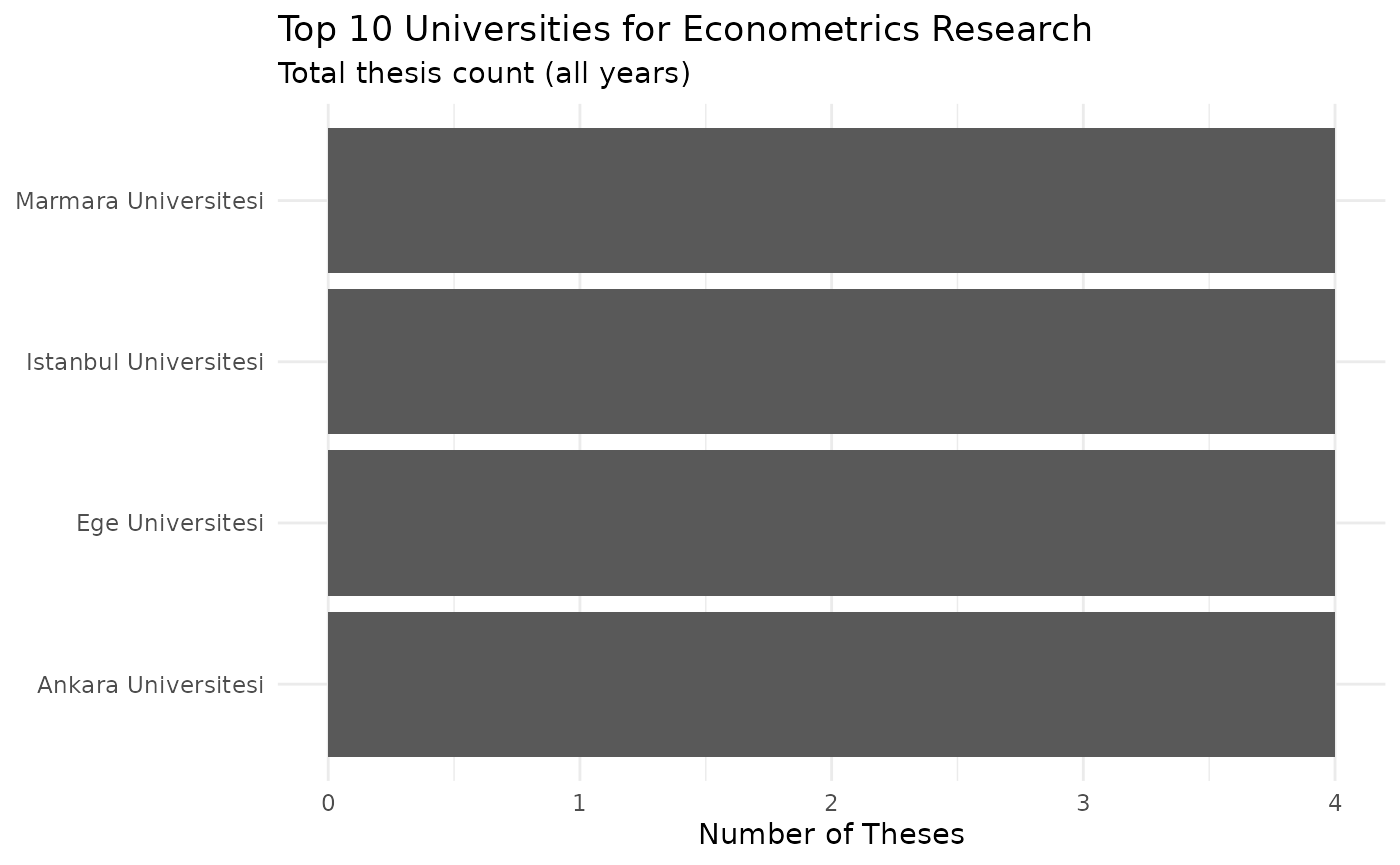
University Trends Over Time
Let’s compare the top four universities from 2000 onward.
top4_unis <- uni_counts$university[1:4]

# Filter to top 4 universities, 2000 onward
uni_trends <- econ_theses |>
  filter(university %in% top4_unis) |>
  mutate(year = as.numeric(year)) |>
  filter(year >= 2000) |>
  count(year, university)

uni_trends |>
  ggplot(aes(x = year, y = n, color = university)) +
  geom_line() +
  labs(
    title = "Econometrics Research Trends at Top Universities",
    subtitle = "2000-present",
    x = "Year",
    y = "Number of Theses",
    color = "University"
  ) +
  facet_wrap(~university, scales = "free_y") +
  theme_minimal(base_size = 11) +
  theme(legend.position = "none")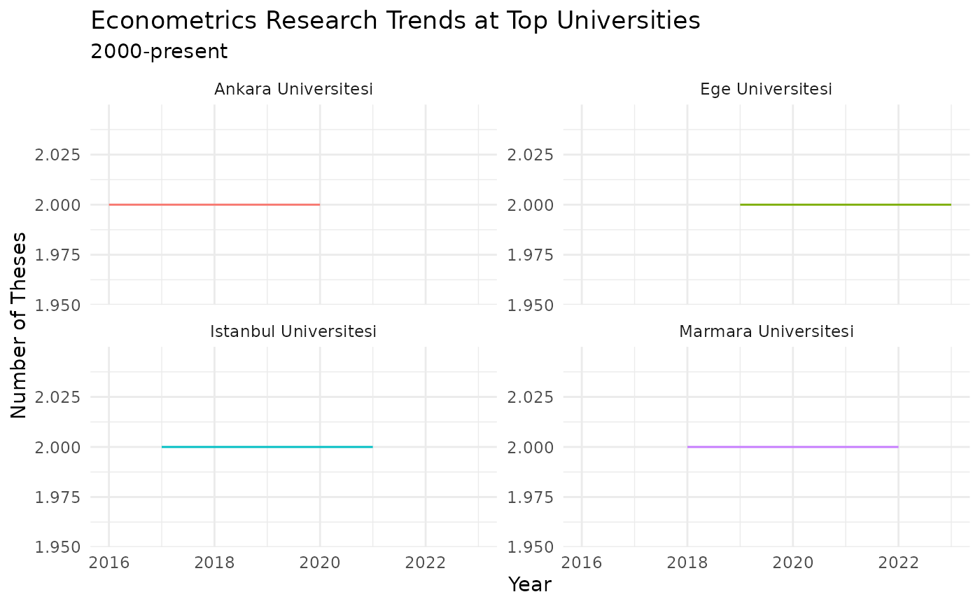
PhD-to-Total Ratio
Let’s assume a higher PhD ratio suggests a more research-intensive program.
# Compute PhD share at each top university
top_unis <- uni_counts$university[1:10]

degree_comparison <- econ_theses |>
  filter(university %in% top_unis) |>
  filter(thesis_type_en %in% c("Master", "Doctorate")) |>
  count(university, thesis_type_en) |>
  pivot_wider(names_from = thesis_type_en, values_from = n, values_fill = 0) |>
  mutate(phd_ratio = Doctorate / (Doctorate + Master)) |>
  arrange(desc(phd_ratio))

degree_comparison
#> # A tibble: 4 × 4
#>   university            Master Doctorate phd_ratio
#>   <chr>                  <int>     <int>     <dbl>
#> 1 Ege Universitesi           0         4         1
#> 2 Istanbul Universitesi      0         4         1
#> 3 Ankara Universitesi        4         0         0
#> 4 Marmara Universitesi       4         0         0
Example 3: Keyword and Abstract Analysis
You can extract research themes from thesis abstracts and keywords.
Detail records include keywords_tr,
keywords_en, abstract_original, and
abstract_translation. This example fetches details for all
matching theses, so it is slow.
Collecting Detailed Metadata
# Search for machine learning theses
if (live_examples) {
  ml_search <- search_basic("makine öğrenmesi",
                            max_search_results = Inf)

  # Fetch full details (abstracts, keywords, advisor, PDF URLs)
  ml_search_sample <- ml_search |>
    slice_sample(n = 20)

  ml_details <- detail(ml_search_sample$detail_id)
} else {
  ml_details <- tezr_example_ml_details()
}

ml_details
#> # A tibble: 5 × 2
#>   thesis_no keywords_tr
#>   <chr>     <chr>
#> 1 910001    Makine ogrenmesi; Derin ogrenme; Siniflandirma
#> 2 910002    Makine ogrenmesi; Yapay zeka; Tahmin
#> 3 910003    Derin ogrenme; Goruntu isleme; Sinir aglari
#> 4 910004    Makine ogrenmesi; Veri madenciligi; Siniflandirma
#> 5 910005    Dogal dil isleme; Makine ogrenmesi; Metin madenciligi
Keyword Frequency
The keywords_tr field contains semicolon separated
terms. Let’s split them, trim whitespace, and count.
# Parse comma-separated keywords into individual rows
keywords <- ml_details |>
  filter(!is.na(keywords_tr)) |>
  select(thesis_no, keywords_tr) |>
  mutate(keywords_tr = str_split(keywords_tr, stringr::fixed(";"))) |>
  unnest(keywords_tr) |>
  mutate(keyword = str_trim(keywords_tr)) |>
  filter(keyword != "")

# Top 5 keywords
keyword_freq <- keywords |>
  count(keyword, sort = TRUE) |>
  head(5)

keyword_freq |>
  ggplot(aes(x = n, y = reorder(keyword, n))) +
  geom_col() +
  labs(
    title = "Most Common Keywords in Machine Learning Theses",
    x = "Frequency",
    y = NULL
  ) +
  theme_minimal(base_size = 11)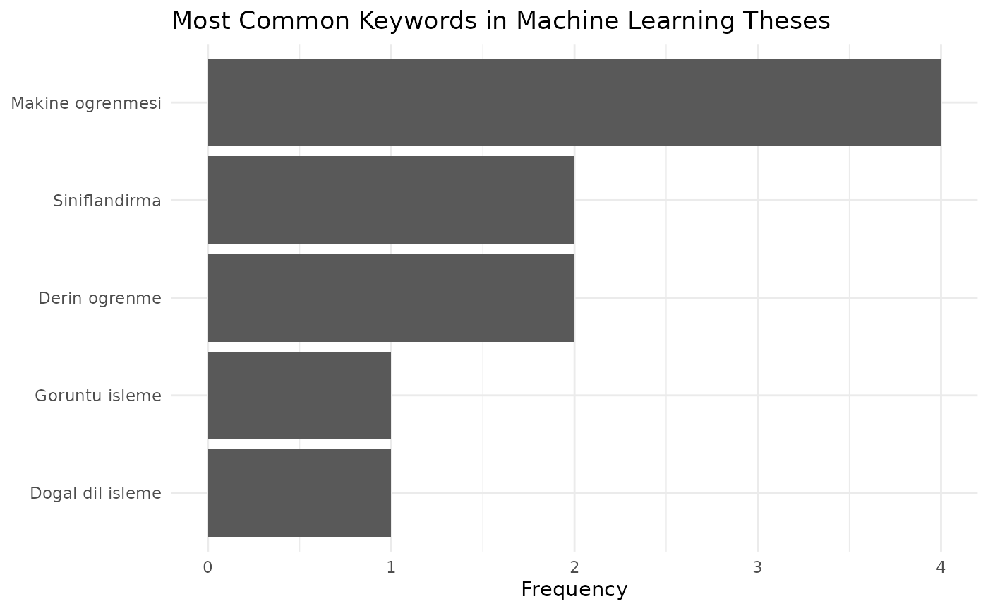
Tips for Large-Scale Analysis
Saving Results Locally
Save search results to disk after the first fetch. Load them in later sessions to skip network calls. RDS preserves column types and CSV is useful for sharing.
Incremental Detail Retrieval
For large result sets, fetch details in batches and save each batch. This protects against interruptions — if the process stops, you only lose the current batch.
batch_size <- 50
all_results <- search_basic("panel data")

for (i in seq(1, nrow(all_results), by = batch_size)) {
  batch_end <- min(i + batch_size - 1, nrow(all_results))
  batch <- all_results[i:batch_end, ]

  # detail() uses built-in rate limiting
  details <- detail(batch$detail_id)

  # Save each batch to disk
  saveRDS(details, paste0("details_batch_", i, ".rds"))

  # Optional short pause between batches
  Sys.sleep(2)
}
Rate Limiting
tezr uses a built-in 2-second rate limit for request setup.
detail() fetches uncached records in parallel (up to 5
active requests), and large jobs can still take time. Process in batches
and cache results when possible.