Downloading and Plotting Maps with tuikr

Introduction

tuikr returns both the indicator values and the matching geometries needed for a map. A typical workflow is:

1. discover a geographic variable with tuikr::geo_data()
2. confirm the available NUTS levels in var_levels
3. download the values for one level
4. join them to tuikr::geo_map()
5. plot the result

Find a Geographic Series

Start in metadata mode and locate the housing-sales series used below.

geo_variable_catalog <- tuikr::geo_data()
geo_variable_catalog_tr <- tuikr::geo_data(lang = "tr")

housing_sales_series <- geo_variable_catalog |>
  dplyr::filter(var_num == "INS-GK055-O006")

housing_sales_series |>
  dplyr::select(
    var_name,
    var_num,
    var_levels,
    var_period
  )
#> # A tibble: 1 × 4
#>   var_name                      var_num        var_levels var_period
#>   <chr>                         <chr>          <list>     <chr>     
#> 1 Number of house sales (total) INS-GK055-O006 <int [1]>  yillik

geo_variable_catalog_tr |>
  dplyr::filter(var_num == "INS-GK055-O006") |>
  dplyr::select(var_name, var_num)
#> # A tibble: 1 × 2
#>   var_name                      var_num       
#>   <chr>                         <chr>         
#> 1 Konut satış sayıları (toplam) INS-GK055-O006

Use lang = "tr" to get Turkish indicator names in the metadata table and in the downloaded value column.

var_levels is a list-column. Pull the first element to inspect the levels available for this series. Use var_level only when a series is published at more than one level.

housing_sales_series$var_levels[[1]]
#> [1] 3

Download the Values

INS-GK055-O006 is published at level 3, which is the provincial map.

housing_sales <- tuikr::geo_data(
  var_num = "INS-GK055-O006",
  var_level = 3
) |>
  dplyr::mutate(
    date = as.integer(date),
    number_of_house_sales_total = as.numeric(number_of_house_sales_total)
  )

housing_sales |>
  dplyr::slice_head(n = 8)
#> # A tibble: 8 × 3
#>   code   date number_of_house_sales_total
#>   <chr> <int>                       <dbl>
#> 1 66     2025                        7732
#> 2 66     2024                        7238
#> 3 66     2023                        6483
#> 4 66     2022                        7504
#> 5 66     2021                        6238
#> 6 53     2025                        3668
#> 7 53     2024                        3569
#> 8 53     2023                        3459

Download the Boundaries

tuikr::geo_map(3) returns an sf object that is already keyed by the code column used in tuikr::geo_data().

province_boundaries <- tuikr::geo_map(3)

province_boundaries |>
  dplyr::select(code, ad) |>
  dplyr::slice_head(n = 6)
#> Simple feature collection with 6 features and 2 fields
#> Geometry type: MULTIPOLYGON
#> Dimension:     XY
#> Bounding box:  xmin: 27 ymin: 36.0798 xmax: 39.2599 ymax: 39.27
#> Geodetic CRS:  WGS 84
#> # A tibble: 6 × 3
#>   code  ad                                                     geometry
#>   <chr> <chr>                                        <MULTIPOLYGON [°]>
#> 1 9     AYDIN          (((28.2497 37.5499, 28.2295 37.5204, 28.2204 37…
#> 2 1     ADANA          (((36.18 37.7096, 36.1898 37.7, 36.1397 37.7, 3…
#> 3 2     ADIYAMAN       (((38.9199 37.8197, 38.9498 37.7999, 38.9602 37…
#> 4 3     AFYONKARAHİSAR (((30.6098 38.2199, 30.55 38.1601, 30.5201 38.1…
#> 5 7     ANTALYA        (((32.1898 36.9604, 32.2399 36.9198, 32.2496 36…
#> 6 20    DENİZLİ        (((28.76 37.2496, 28.7295 37.2698, 28.7295 37.3…

If you only want the attribute table, call tuikr::geo_map(level = 3, dataframe = TRUE).

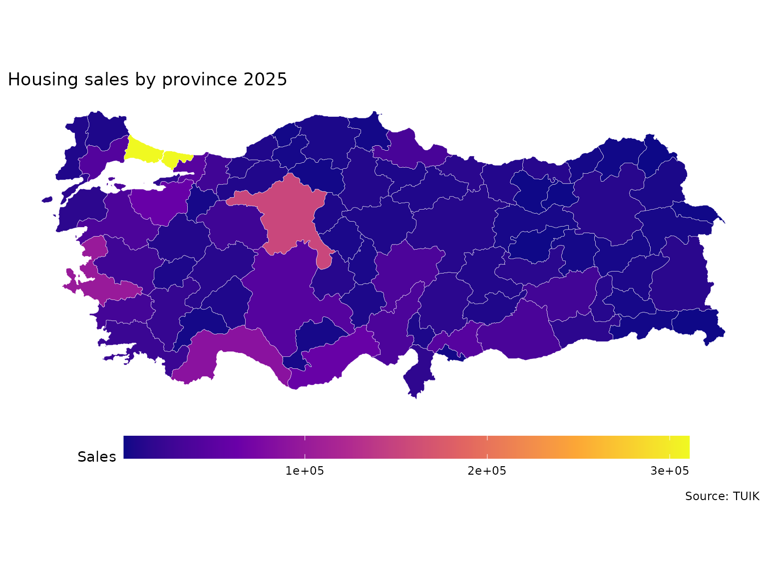
Join and Plot

Filter to the latest available year, join on code, and plot the result.

latest_year <- max(housing_sales$date, na.rm = TRUE)

housing_sales_latest <- housing_sales |>
  dplyr::filter(date == latest_year)

housing_sales_map <- province_boundaries |>
  dplyr::left_join(housing_sales_latest, by = "code")

ggplot2::ggplot(housing_sales_map) +
  ggplot2::geom_sf(
    ggplot2::aes(fill = number_of_house_sales_total),
    color = "white",
    linewidth = 0.1
  ) +
  ggplot2::coord_sf(datum = NA) +
  ggplot2::scale_fill_viridis_c(option = "plasma", na.value = "grey90") +
  ggplot2::theme_minimal() +
  ggplot2::theme(
    legend.position = "bottom",
    legend.key.width = grid::unit(3, "cm")
  ) +
  ggplot2::labs(
    title = paste("Housing sales by province", latest_year),
    fill = "Sales",
    caption = "Source: TUIK"
  )

Troubleshooting

If a request fails, go back to the metadata table and inspect var_levels before changing var_level. Many indicators are not available at every geographic level.

If the join produces missing fills, inspect the boundary keys with sf::st_drop_geometry(province_boundaries) or call tuikr::geo_map(level = 3, dataframe = TRUE) to compare codes directly.

If you need a different geometry type, remember that levels 2, 3, and 4 return polygon boundaries while level 9 returns settlement points.